This session focuses on fitting models, building directly on the models used in previous chapters. The session is structured in three parts of roughly 60 minutes each:
Introduction
Determining what model should be used for your problem is only step one in modelling infectious diseases. The next step, which can often be the hardest, is determining the value of your unknown parameters. Sometimes, a thorough literature search may help with understanding the value of a parameter, but often it is up to the researcher to obtain data and determine which parameter values give the best fit. The focus of the next two sessions is to give you practical experience in fitting infectious disease models to data.
Frequentist vs Bayesian Statistics (an overview)
Statistics consists of two main approaches, Frequentist statistics and Bayesian statistics. Often, a statistician will claim to be a Frequentist or a Bayesian, but in my opinion, you should know both points of view and be aware what the implications are.
Frequentist statistics is commonly taught across many degrees at university, being used for \(p\)-values and hypothesis testing. Bayesian statistics is taught later, often in final year mathematics degrees or masters courses. But what is the real difference?
There is one main distinction that you must remember when talking about the difference between Bayesian and Frequentist probability. This distinction is entirely to do with how you want to view the world. Frequentist statistics says that the data is a random variable given the parameters. Therefore, if you repeat your data generating process (such as an experiement or survey), the underlying parameters are the same but you will observe a different outcome. Bayesian statistics says that the parameters are random variables given the data. This implies that the data you have seen is the data, we do not ask the question of repeating the data generating process, and the underlying parameters that generated the data are uncertain and from a distribution.
More succinctly, Frequentists love and use the likelihood \[
p(D|\theta),
\] where \(D\) is the data and \(\theta\) is the parameters of interest, and Bayesians love the posterior \[
p(\theta|D).
\]
Are we done? Yes. Is there so much more to it than that super simple explanation? Yes.
Note
Let us run a survey. Who is a Bayesian? Who is a Frequentist?
An example?
Let us now demonstrate a key difference between frequentist and bayesian statistics using \(p\)-values. We will start by investigating an extremely simple model of trying to determine the mean of a normal distribution.
Let us say that we have measured 20 data points that we believe are normally distributed with an unknown mean, \(\mu\) but a known variance, \(\sigma^2\). When we think like a frequentist, we look at our data (which we believe is sampled from a distribution) and we determine an estimate for our mean. This is typically done using maximum likelihood. This is it, we are done, we have our measurement for the mean. It is, \[
\hat{\mu} = \frac{1}{20}\sum_{i=1}^{20} D_i
\] where \(D_i\) is our \(i\)-th data point and \(\hat{\mu}\) is our estimate of the true mean.
But as a frequentist, we might then say… well that was our measurement but “Is it a significant measurement!”
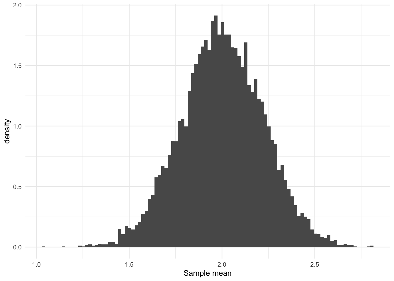
To look at significance, we actually look at the distribution of the maximum likelihood estimate. Wait, a distribution of the maximum likelihood? That does not make sense as it is a point. Yes it is a point estimate, but what we do is we look at how that point estimate will change BECAUSE OUR DATA IS RANDOM.
The next time we collect data, we expect that we will get a different point estimate of the mean! What is the distribution? Well, \[
D_i \sim \mathcal{N}(\mu,\sigma^2),
\] where \(\mathcal{N}\) is used to denote the normal distribution, so we have that \[
\hat{\mu} = \frac{1}{20}\sum_{i=1}^{20} D_i \sim \mathcal{N}(\mu, \frac{\sigma^2}{20}).
\] So because the data varies our estimate for the maximum likelihood is also a random variable! If you do not believe me, lets look at this example
This calculates the repeated sample means that result from our varying data.
The point of p-values is to now ask the question. Given the model assumptions that we have made, what is the probability that I observed my estimated mean?
As a bayesian, we would not consider repeating the experiment over and over to determine a distribution of sample means. Instead we would use Baye’s Theorem to determine the probability distribution for the true mean. We would look at \[
p(\mu |D) \propto p(D|\mu)p(\mu),
\] where \(p(\mu|D)\) is called the posterior, \(p(D|\mu)\) is our likelihood (which is the same as the likelihood used in a frequentist version) and \(p(\mu)\) is our prior distribution. The prior distribution is of interest as it is encodes our prior belief in the value of \(\mu\) before we observed the data. If we continue with our previous example we would say that \[
p(D|\mu) = \prod_{i=1}^{20} \mathcal{N}(D_i | \mu, \sigma^2) = (2 \pi \sigma^2)^{-20/2}\exp\left(-\frac{20}{2\sigma^2}(\bar{D} - \mu)^2\right)
\] where \(\bar{D}\) is the emirical mean of the data. We could say that our prior belief is that \(\mu\) is around zero, through, \[
p(\mu) = \mathcal{N}(\mu|0,\lambda^2)
\] where \(\lambda\) is the variance we expect in our prior belief around \(\mu\). Having defined all of this, the distribution for our mean is (using Bayes’ Theorem, which we will get to), \[
\begin{aligned}
p(\theta|D) &\propto \prod_{i=1}^{20} \mathcal{N}(D_i | \mu, \sigma^2)\mathcal{N}(\mu|0,\lambda^2) \nonumber \\
&\propto \exp\left(-\frac{20}{2\sigma^2}( \bar{D} - \mu)^2 -\frac{\mu^2}{2\lambda^2}\right) \\
&\propto \exp\left(-\frac{20}{2\sigma^2}\mu^2 -\frac{20}{2\sigma^2}2 \bar{D} \mu -\frac{\mu^2}{2\lambda^2}\right) \\
&\propto \exp\left(-\frac{20\lambda^2 + \sigma^2}{2\sigma^2\lambda^2}\left(\mu^2 -2 \frac{20\lambda^2}{20 \lambda^2 + \sigma^2} \bar{D} \mu -\frac{\mu^2}{2\lambda^2}\right)\right) \\
&\propto \exp\left(-\frac{20\lambda^2 + \sigma^2}{2\sigma^2\lambda^2}\left(\mu -\frac{20\lambda^2}{20 \lambda^2 + \sigma^2} \bar{D}\right)^2\right)
\end{aligned}
\]
Note
The posterior in the above example, \(p(\theta |D)\), is a normal distribution where \[
\frac{20\lambda^2}{20 \lambda^2 + \sigma^2} \bar{D},
\] is the mean and \[
\frac{\sigma^2\lambda^2}{20\lambda^2 + \sigma^2},
\] is the variance! The full derivation is a fun piece of algebra that you should check yourself.
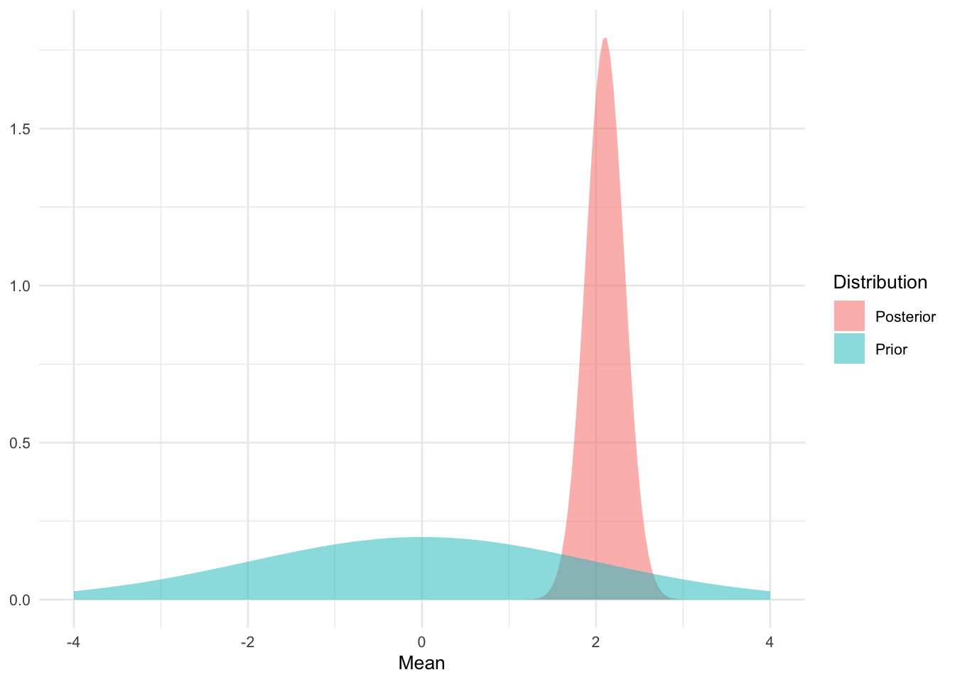
Now that is the answer from a Bayesian perspective - we have determined our distribution of belief in \(\mu\) after observing our data. We do not ask the same \(p\)-value questions as before as it does not have any meaning to us. The data that we measured updated our belief for what we think the value of \(\mu\) is.
Often people consider frequentist statistics as bayesian statistics without the use of a prior. This is not the case, it is a fundamental shift in how we want to interpret our data.